Macro Letter – No 36 – 22-05-2015
Rising yields and rising correlation in major bond markets – end of cycle or correction?
- European bond yields have risen following the lead of US treasuries
- Yield curves are steepening despite minimal inflation
- A return to the natural rate of interest seems unlikely
- Over-indebtedness will stifle GDP growth and yields will fall
Since the beginning of 2015 the world’s largest bond markets have witnessed increasing yields. In the aftermath of the Great Financial Crisis many economies decoupled and their government bond markets followed suit. Now correlations are rising once more. The table below, which is a snapshot of prices on Tuesday morning 19th May, looks at a broad range of developed bond markets:-
| Bond & Maturity |
Yield |
Low |
Date |
Change |
CPI |
Real yield |
10yr-2yr |
| Australia 2Y |
2.035 |
|
|
|
|
|
|
| Australia 5Y |
2.305 |
|
|
|
|
|
|
| Australia 10Y |
2.92 |
2.236 |
March |
0.684 |
1.3 |
1.62 |
0.885 |
| Canada 2Y |
0.646 |
|
|
|
|
|
|
| Canada 5Y |
1.006 |
|
|
|
|
|
|
| Canada 10Y |
1.711 |
1.23 |
February |
0.481 |
1.2 |
0.511 |
1.065 |
| Denmark 2Y |
-0.299 |
|
|
|
|
|
|
| Denmark 5Y |
0.088 |
|
|
|
|
|
|
| Denmark 10Y |
0.786 |
0.075 |
February |
0.711 |
0.5 |
0.286 |
1.085 |
| France 2Y |
-0.162 |
|
|
|
|
|
|
| France 5Y |
0.182 |
|
|
|
|
|
|
| France 10Y |
0.832 |
0.332 |
April |
0.5 |
0.1 |
0.732 |
0.994 |
| Germany 2Y |
-0.21 |
|
|
|
|
|
|
| Germany 5Y |
0.026 |
|
|
|
|
|
|
| Germany 10Y |
0.563 |
0.049 |
April |
0.514 |
0.5 |
0.063 |
0.773 |
| Italy 2Y |
0.108 |
|
|
|
|
|
|
| Italy 5Y |
0.697 |
|
|
|
|
|
|
| Italy 10Y |
1.753 |
1.041 |
March |
0.712 |
-0.1 |
1.853 |
1.645 |
| Japan 2Y |
-0.002 |
|
|
|
|
|
|
| Japan 5Y |
0.103 |
|
|
|
|
|
|
| Japan 10Y |
0.388 |
0.199 |
January |
0.189 |
2.3 |
-1.912 |
0.39 |
| New Zealand 2Y |
3.09 |
|
|
|
|
|
|
| New Zealand 5Y |
3.25 |
|
|
|
|
|
|
| New Zealand 10Y |
3.74 |
3.085 |
January |
0.655 |
0.1 |
3.64 |
0.65 |
| Norway 2Y |
0.857 |
|
|
|
|
|
|
| Norway 5Y |
1.035 |
|
|
|
|
|
|
| Norway 10Y |
1.676 |
1.202 |
February |
0.474 |
2 |
-0.324 |
0.819 |
| Sweden 2Y |
-0.331 |
|
|
|
|
|
|
| Sweden 5Y |
0.169 |
|
|
|
|
|
|
| Sweden 10Y |
0.691 |
0.216 |
April |
0.475 |
-0.2 |
0.891 |
1.022 |
| Switzerland 2Y |
-0.839 |
|
|
|
|
|
|
| Switzerland 5Y |
-0.48 |
|
|
|
|
|
|
| Switzerland 10Y |
-0.003 |
-0.28 |
January |
0.281 |
-1.1 |
1.097 |
0.836 |
| UK 2Y Yield |
0.537 |
|
|
|
|
|
|
| UK 5Y Yield |
1.39 |
|
|
|
|
|
|
| UK 10Y Yield |
1.892 |
1.337 |
January |
0.555 |
-0.1 |
1.992 |
1.355 |
| US 2Y Yield |
0.565 |
|
|
|
|
|
|
| US 5Y Yield |
1.506 |
|
|
|
|
|
|
| US 10Y Yield |
2.193 |
1.63 |
January |
0.563 |
-0.1 |
2.293 |
1.628 |
Source: Investing.com and Trading Economics
I’ve highlighted some of the data. The highest real 10yr yield is to be found in New Zealand (3.64%) but US T-Bonds lie second. The lowest real yield is evident in Japanese Government Bonds (JGBs) however, a quick glance at the shape of the Japanese yield curve suggests that inflation, or perhaps I should say deflation, expectations are firmly anchored at near zero, despite repeated bouts of Abenomic stimulus. Japan has the flattest yield curve. The US curve is second steepest, behind Italy, where the spread between 2yr and 10yr is 164.5bp. Italy has also seen the largest rise in yields since its low back in March, although Danish yields have risen to a similar degree as its non-Euro “safe haven” status has waned.
A number of factors have driven yields higher. In the Eurozone (EZ) concern about a Greek exit initially stimulated a “flight to safety” in government securities – other than Greek government bonds – this spilled over into Swiss Confederation bonds. Switzerland remains the ultimate “safe haven”. As yields in the EZ declined to record lows, capital also flowed into EZ stocks. At the same time economic data began to turn more positive, prompted further flows into equities. The last EZ bond markets to turn lower were France and Germany, last month.
Outside the EZ, the US economy has seen mixed data but GDP growth remains steady. Expectations of Federal Reserve rate increases, whilst still some way off (current consensus January 2016) weigh on the T-Bond market. A rebound in crude oil and weakening of the US$ TWI since its highs in early March have also seen an unwinding of bullish US$ and US Treasury exposures.
Stock markets have so far paid little heed to the bond markets. The S&P500 made new highs this week. Canada, Japan, Germany and the UK all made highs in April whilst the Australian ASX retouched its March highs during the month. Even New Zealand, with the second flattest yield curve and structurally higher real interest rate curve, is less than 4% off its all-time highs.
Inflation expectations and real returns
Earlier this week saw the publication of this first part of a two part article about inflation expectations from the NY Fed – FRBNY DSGE Model Forecast–April 2015:-
The top panel in the chart below presents quarterly forecasts for real output growth and the core PCE inflation rate over the 2014-17 horizon. These forecasts were produced on April 9 using data released through 2014:Q4, augmented for 2015:Q1 with a “nowcast” for GDP growth, core PCE inflation, and growth in total hours, and 2015:Q1 observations for financial variables. The reason for using nowcasts is that the model is estimated on National Income and Product Accounts data, which are only available with a lag. Nowcasts incorporate up-to-date information, and this tends to improve short-run forecasts, as shown here. The black line represents released data, the red line is the forecast, and the shaded areas mark the uncertainty associated with our forecasts at 50, 60, 70, 80, and 90 percent probability intervals. Output growth and inflation are expressed in quarter-to-quarter percentage annualized rates.

Source: NY Fed
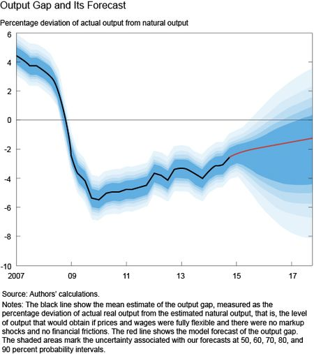
The FRBNY DSGE forecast for output growth is slightly stronger than it was in our earlier blog post which used data ending in July 2014. This difference is highlighted in the bottom left panel of the chart, which compares current (solid line) and September (dashed line) forecasts. The model projects the economy to grow 1.9 percent in 2015 (Q4/Q4), 2.1 percent in 2016 and 2.2 percent in 2017. The headwinds that slowed down the economy in the aftermath of the financial crisis are finally abating. This is reflected in the model-implied “natural” level of output and the “natural” rate of interest, which are defined as the counterfactual level of output and interest rate that would obtain in an ideal economy where nominal rigidities, markup (or cost-push) shocks, and financial frictions are absent. Estimates of the recent natural level of output show a more rapid growth as the headwinds facing the economy are fading. As we will discuss at length in our next post, the natural rate of interest is finally increasing toward positive ranges, after having been negative for the entire post-Great Recession period. The recovery has been relatively slow, however, with economic activity remaining below its natural level since the end of 2008 and projected to remain so throughout the forecast horizon. The model thus predicts a very gradual closing of the output gap, measured as the percentage deviation of actual output from natural output (although there is much uncertainty about the gap forecast). This output gap, along with its forecast, is shown in the next chart.

Source: NY Fed
…In conclusion, the FRBNY DSGE model continues to predict a gradual recovery in economic activity with a slow return of inflation toward the FOMC’s long-run target of 2 percent, as the negative effect of the Great Recession dissipates. This forecast remains surrounded by significant uncertainty, with the risks slightly skewed to the downside for output growth because of the constraint on policy imposed by the zero lower bound.
The Peterson Institute – Quantity Theory of Money Redux? Will Inflation Be the Legacy of Quantitative Easing? Examines the classical monetarist argument that QE will eventually lead to inflation, this is their conclusion:-
On balance, the risk of severe inflation resulting from the buildup of the balance sheet of the Federal Reserve in association with quantitative easing seems low. To begin with, the US economy has not experienced inflation driven by excessive money expansion since at least the mid-1980s. Indeed, the rising demand for money, as the opportunity cost of holding money fell with lower inflation, has meant that over the past three decades there has been a tendency for faster money growth(relative to real GDP) to be associated with lower rather than higher inflation. The supply-focused quantity theory of money broke down. The pattern associating rapid money growth with low inflation since the mid-1980s would require a sharp reversal for money supply to become the proximate cause of inflation. In the meantime, it seems fair to say that in the United States inflation is determined by labor market and product market tightness (in the Phillips curve tradition), and that the opposing proposition that “inflation is always and everywhere a monetary phenomenon” (Friedman’s summary of the quantity theory) does not hold in a narrow sense relating to money supply.
A second important phenomenon is that inflation has remained low despite a large buildup in the Fed’s balance sheet not because the velocity of broad money has collapsed, but because the money multiplier has done so. Because of a large increase in excess bank reserves equal to nearly three-fourths of the increase in the Federal Reserve’s total assets, the usual money multiplier (inverse of the reserve requirement ratio) no longer holds. Broad money was 14 times the money base in 2007; by end-2014 it was only 4 times the money base.
A third observation is that arguably this same phenomenon could pose a risk of inflationary money expansion when and if banks start to draw down excess reserves.
Fourth, the principal implication for policy purposes is that the Federal Reserve will need to be particularly adept in avoiding any inflationary pressures that might develop from the unwinding of large excess bank reserves as more normal monetary conditions return. The Fed has clearly given considerable attention to this task and at present plans to use higher interest rates on excess reserves as needed to control such pressures. Indeed, the authority to pay interest on reserves is what will enable the Fed to raise rates when necessary, because otherwise an incipient rise in the short-term interest rate would quickly be choked off as banks ran down excess reserves to take advantage of the higher interest rates.
Fifth, because quantitative easing constitutes navigating in uncharted waters, there is some non-zero probability that inflation could nevertheless still be the consequence of potential money supply expansion resulting from QE.
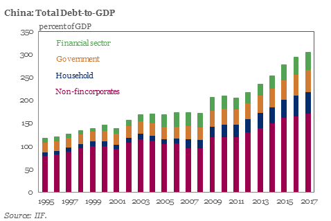
The key element in their assessment is the “multiplier effect”, bank reserve requirements have increased globally since 2008, QE has merely offset the tightening of credit conditions, but in the process it has crowded out the private sector – which is where real-GDP growth is generated.
A more deflationary view of the current environment is provided in the quarterly letter from Hoisington Asset Management, here are Lacy Hunt’s six characteristics of highly over-indebted nations:-
1. Transitory upturns in economic growth, inflation and high-grade bond yields cannot be sustained because debt is too much of a constraint on economic activity.
2. Due to inherently weak aggregate demand, economies are subject to structural downturns without the typical cyclical pressures such as rising interest rates, inflation and exhaustion of pent-up demand.
3. Deterioration in productivity is not inflationary but just another symptom of the controlling debt influence.
4. Monetary policy is ineffectual, if not a net negative.
5. Inflation falls dramatically, increasing the risk of deflation.
6. Treasury bond yields fall to extremely low levels.
…Many assume that economies can only contract in response to cyclical pressures like rising interest rates and inflation, fiscal restraint, over-accumulation of inventories, or the stock of consumer and corporate capital goods. This idea is valid when debt levels are normal but becomes problematic when debt is excessively high.
Large parts of Europe contracted last year for the third time in the past four years as interest rates and inflation plummeted. The Japanese economy has turned down numerous times over the past twenty years while interest rates were low. Indeed, this has happened so often that nominal GDP in Japan is currently unchanged for the past twenty-three years. This is confirmation that after a prolonged period of taking on excessive debt additional debt becomes counterproductive.
…Falling productivity does not cause faster inflation. The weaker output per hour is a consequence of the over-indebtedness as much as the other five characteristics mentioned above. Productivity is a complex variable impacted by many cyclical and structural influences. Productivity declines during recessions and declines sharply in deep ones.
…Monetary policy impacts the overall economy in two areas – price effects and quantity effects. Price effects, or changes in short-term interest rates, are no longer available because rates are near the zero bound. This is a result of repeated quantitative easing by central banks. It is an attempt to lift overly indebted economies by encouraging more borrowing via low interest rates, thus causing even greater indebtedness.
Quantity effects also don’t work when debt levels are excessive. In a non-debt constrained economy, central banks have the capacity, with lags, to exercise control over money and velocity. However, when the debt overhang is excessive, they lose control over both money and velocity. Central banks can expand the monetary base, but this has little or no impact on money growth.
…In periods of extreme over-indebtedness Treasury bond yields can fall to exceptionally low levels and remain there for extended periods. This pattern is consistent with the Fisher equation that states the nominal risk-free bond yield equals the real yield plus expected inflation (i=r+E*). Expected inflation may be slow to adjust to reality, but the historical record indicates that the adjustment inevitably occurs.
The Fisher equation can be rearranged algebraically so that the real yield is equal to the nominal yield minus expected inflation (r=i–E*). Understanding this is critical in determining how unleveraged investors fare. Suppose that this process ultimately reduces the bond yield to 1.5% and expected inflation falls to -1%. In this situation the real yield would be 2.5%. The investor would receive the 1.5% coupon but the coupon income would be supplemented since the dollars received will have a greater purchasing power. A 1.5% nominal yield with real income lift might turn out to be an excellent return in a deflationary environment. Contrarily, earnings growth is problematic in deflation. Businesses must cut expenses faster than the prices of goods or services fall.
Hunt goes on to predict that yields may rise but this presents an opportunity to buy rather than signalling the end of the bond bull market.
A slightly contrasting view is expressed by Bill Gross in Janus Capital – Investment Outlook:-
Because of this stunted growth, zero based interest rates, and our difficulty in escaping an ongoing debt crisis, the “sense of an ending” could not be much clearer for asset markets. Where can a negative yielding Euroland bond market go once it reaches (–25) basis points? Minus 50? Perhaps, but then at some point, common sense must acknowledge that savers will no longer be willing to exchange cash Euros for bonds and investment will wither. Funny how bonds were labeled “certificates of confiscation” back in the early 1980’s when yields were 14%. What should we call them now? Likewise, all other financial asset prices are inextricably linked to global yields which discount future cash flows, resulting in an Everest asset price peak which has been successfully scaled, but allows for little additional climbing. Look at it this way: If 3 trillion dollars of negatively yielding Euroland bonds are used as the basis for discounting future earnings streams, then how much higher can Euroland (Japanese, UK, U.S) P/E’s go? Once an investor has discounted all future cash flows at 0% nominal and perhaps (–2%) real, the only way to climb up a yet undiscovered Everest is for earnings growth to accelerate above historical norms. Get down off this peak, that F. Scott Fitzgerald once described as a “Mountain as big as the Ritz.” Maybe not to sea level, but get down. Credit based oxygen is running out.
But what should this rational investor do? Breathe deeply as the noose is tightened at the top of the gallows? Well no, asset prices may be past 70 in “market years”, but savoring the remaining choices in terms of reward / risk remains essential. Yet if yields are too low, credit spreads too tight, and P/E ratios too high, what portfolio or set of ideas can lead to a restful, unconscious evening ‘twixt 9 and 5 AM? That is where an unconstrained portfolio and an unconstrained mindset comes in handy. 35 years of an asset bull market tends to ingrain a certain way of doing things in almost all asset managers. Since capital gains have dominated historical returns, investment managers tend to focus on areas where capital gains seem most probable. They fail to consider that mildly levered income as opposed to capital gains will likely be the favored risk / reward alternative. They forget that Sharpe / information ratios which have long served as the report card for an investor’s alpha generating skills were partially just a function of asset bull markets. Active asset managers as well, conveniently forget that their (my) industry has failed to reduce fees as a percentage of assets which have multiplied by at least a factor of 20 since 1981. They believe therefore, that they and their industry deserve to be 20 times richer because of their skill or better yet, their introduction of confusing and sometimes destructive quantitative technologies and derivatives that led to Lehman and the Great Recession.
Hogwash. This is all ending. The successful portfolio manager for the next 35 years will be one that refocuses on the possibility of periodic negative annual returns and miniscule Sharpe ratios and who employs defensive choices that can be mildly levered to exceed cash returns, if only by 300 to 400 basis points. My recent view of a German Bund short is one such example. At 0%, the cost of carry is just that, and the inevitable return to 1 or 2% yields becomes a high probability, which will lead to a 15% “capital gain” over an uncertain period of time. I wish to still be active in say 2020 to see how this ends. As it is, in 2015, I merely have a sense of an ending, a secular bull market ending with a whimper, not a bang. But if so, like death, only the timing is in doubt. Because of this sense, however, I have unrest, increasingly a great unrest. You should as well.
I believe the world’s major central banks still have the capacity to provide support, should the bond and stock markets collapse, by the effective “quasi-nationalisation” of assets – both equity and fixed income, but I foresee a point where there is a public challenge to the legality of this activity as it crowds out the private sector. I also expect that investors will eventually realise that income generating assets must offer a real-return regardless of potential capital appreciation.
In aggregate, trading is a zero-sum game – except for the broker – investing, by contrast, is about generating long-term income. In a deflationary environment a government bond, should it prove to be risk-free, may offer good value even at next to the zero bound, but, for less fortunate bond holders, default risk needs to be compensated. What is a fair price for lending money to a grateful government? The Minneapolis Fed – Sovereign Default: The Role of Expectations takes a fresh approach to some of these issues. Thomas Piketty – Capital in the 21st Century suggests 5% is the long-term average return on investment, based on his extensive historical research – the link is to a Pdf presentation from 2014, which is easier than reading the 700 page book. Given developed nation governments propensity to run budget deficits, this seems a reasonable return. The only government offering close to 5% is New Zealand at 3.74%. Ironically, their Debt to GDP ratio is only 36% and they have run a small budget surplus for most of the last 40 years.
If risk premia are not permitted to return towards their long-run average, I envisage liquidity disappearing from bond and stock markets as public institutions – namely central banks – acquire the majority of bond issues and the free-float in “strategically important” stocks. Crowdfunding and microfinance may fill some of the gap and capital will flow to growing economies as the world order changes, but liquidity in the world’s largest capital markets may be in short supply. Fortunately, this somewhat apocalyptic view is a while away.
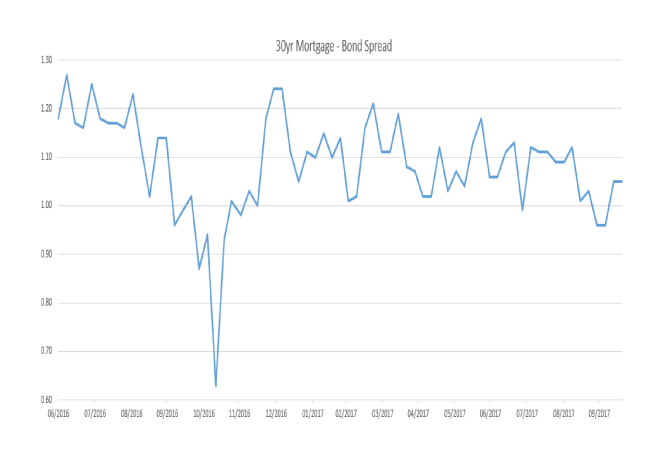
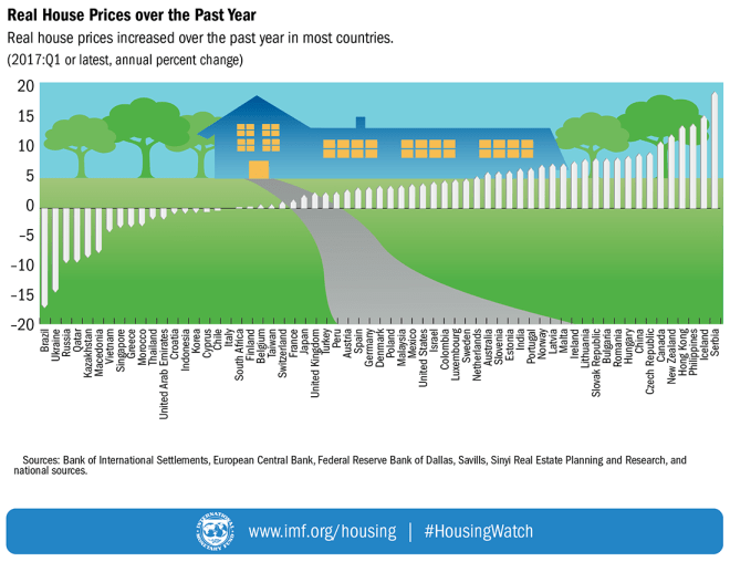
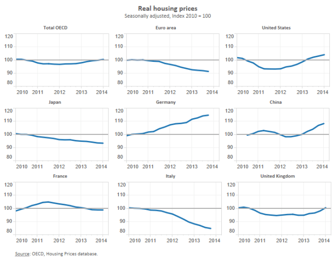
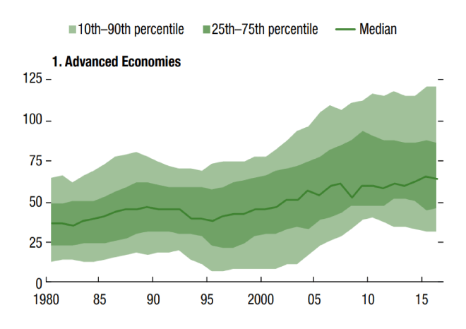
Bond yields may rise, but not significantly above 5%, at which juncture their respective economies will stall due to over-indebtedness – in reality I think it unlikely they will get anywhere near this level until pricing power in product markets returns. The FRBSF – Mortgaging the Future? Investigates the extraordinary expansion in credit since WWII and among their conclusions is the observation that the real estate sector has far greater impact on the economy than in the past. Of course the absolute return to savers is likely to remain pitiful, as this video, from the March conference of the Global Interdependence Centre – Policies for the Post Crisis Era, makes clear; Chris Whalen’s presentation starts around 4 minutes in and lasts for 10 minutes. It’s well worth considering his opinion that, for the world economy to function properly, interest rates need to rise and credit formation to rebound, lest the “wheel of circulation” – as originally described by Adam Smith – grind to an inexorable halt.
For most of the major Central banks, intervention will be undertaken if yield increases are deemed to be detrimental to the mortgage market, and, as bond yields then trend lower, stocks will rise.
At what rate will they intervene? The NY Fed recently commented on “the natural rate of interest” is this article – Why Are Interest Rates So Low?:-
In conclusion, the low level of interest rates experienced since 2008 is largely attributable to a reduction in the natural rate of interest, which reflects cautious behavior on the part of households and firms. Monetary policy has largely accommodated the decline in the natural rate of interest, in order to mitigate the adverse effects of the crisis, but the zero lower bound on interest rates has imposed a constraint on the ability of interest rate policy to stabilize the economy. Looking ahead, we expect these headwinds to continue to abate, and the natural rate of interest to return closer to historical levels.
This is somewhat at odds with thier DSGE forecast. Consensus indicates the natural rate of interest to be around 3% which equates to a nominal rate of 5% assuming an inflation target of 2%. The original concept of the natural rate of interest was introduced in 1898 by Knut Wicksell, it’s a slippery customer:-
…it is not a high or low rate of interest in the absolute sense which must be regarded as influencing the demand for raw materials, labour, and land or other productive resources, and so indirectly as determining the movement of prices. The causality factor is the current rate of interest on loans as compared to [the natural rate].
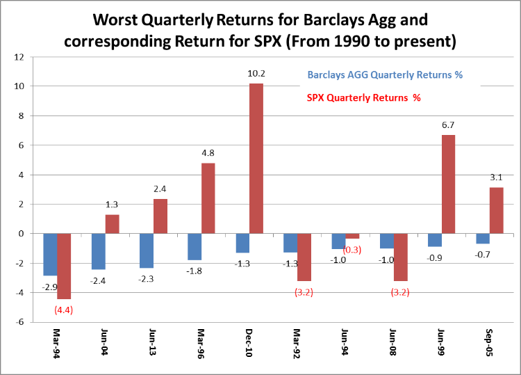
In the shorter term I do not believe bond investors will suffer too catastrophically. I’m indebted to Garth Friesen – III Capital Management –for the excellent charts below:-

Source: III Capital Management
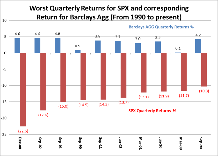
You can read his assessment of the current situation in this article – Silencing the Roar of the Bond Bear. In the past 25 years the largest negative quarterly return from the Barclays bond index was -2.9%, that was back in 1994 when the Fed tightened interest rates abruptly, causing stocks and bonds to collapse in tandem. The next chart highlights the benefits of diversification, generally bonds flip when stocks flop:-

Source: III Capital Management
Conclusion and investment opportunities
If inflation is likely to remain subdued due to the excessive debt overhang, then the recent rise in bond prices is simply a correction. How far will this correction go or has it already run its course?
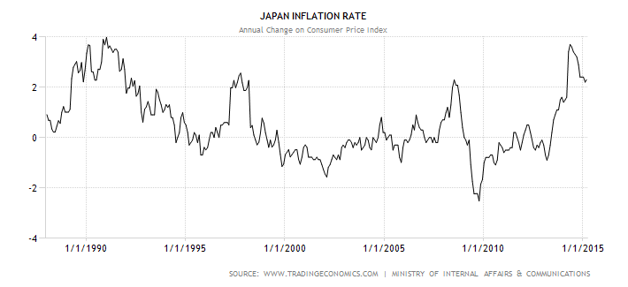
I could analyse each market, apply an array of technical analysis and establish a set of individual forecasts but I believe it is better to view these markets through the lens of the JGB market. Japan has been struggling with bouts of deflation since the 1990’s. Whilst most other nations – Switzerland being a notable exception – have only recently witnessed widespread falling prices, the evolution of inflation expectations are likely to follow a similar course.

Source: Trading Economics and Japanese Ministry of Internal Affairs

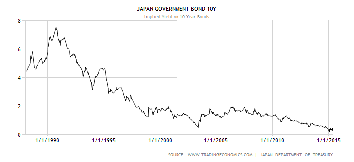
Source: Trading Economics and Japanese Treasury

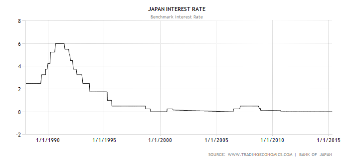
Source: Trading Economics and Bank of Japan
As the Japanese stock market collapsed after 1989 inflation declined rapidly. JGBs, influenced by the rate tightening of the US Fed, suffered a rise in yields in 1994 but then declined once more – after all, the price index was now negative. Inflation witnessed a brief rebound ahead of the Asian Financial Crisis of 1998. The Bank of Japan (BoJ) left short term interest rates on hold and JGB yields declined again as the Asian Crisis gathered momentum.
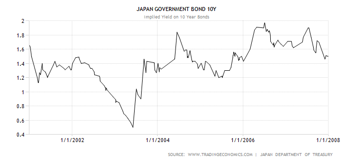
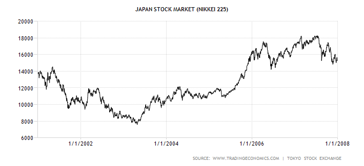
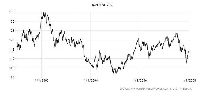
Between 2000 and 2005 Japan struggled with mild deflation, despite expansionary monetary and fiscal policies. At the risk of being vilified for wild generalisation, this is the point where the other bond markets are now. The charts below cover the period 2001-2007, after the bursting of the US Technology Bubble and prior to the Sub-Prime collapse:-

Source: Trading Economics and Japanese Treasury

Source: Trading Economics and Tokyo Stock Exchange

Source: Trading Economics
The table below extrapolates the corrections and counter-corrections of the JGB in the chart above and compares them to the German Bund and the US Treasury 10 year maturities:-
| JGB 10yr |
Rise/Fall |
Change |
Bund 10yr |
Rise/Fall |
Change |
US T-Bond 10yr |
Rise/Fall |
Change |
| Range in bp |
BP |
% |
Equivalent bp |
BP |
% |
Equivalent bp |
BP |
% |
| 55 – 185* |
130* |
236* |
5 – 80* |
75* |
1500* |
138 – 304* |
166* |
120* |
| 185 – 120* |
-65* |
-35* |
80 – 52 |
-28 |
35 |
304 – 163* |
-141* |
-46* |
| 120 – 195* |
75* |
63* |
52 – 85 |
33 |
63 |
163 – 266 |
103 |
63 |
| 195 – 160* |
-35* |
-18* |
85 – 70 |
-15 |
-18 |
266 – 218 |
-48 |
-18 |
| 160 – 190* |
30* |
19* |
70 – 83 |
13 |
19 |
218 – 259 |
41 |
19 |
*These figures are actual outcomes
Source: Investing.com and Tokyo Stock Exchange
I am taking the US T-Bond low (1.38%) of July 2012 to be the current nadir. It may now be embarking on a third corrective wave, if you believe in Elliott Wave theory, which could see yields rise toward 3% once more. The Bund correction, from 80bp to 55bp by 19th May, was probably too swift, meaning the market may break above 0.80% before yields decline again.
The price cycles in each of these markets are unlikely to tally either in duration or magnitude, but, after a capitulation in Europe, in which 10yr Bund yield almost turned negative, even the most ardent fixed income protagonists have been unable to justify remaining fully invested – we have now entered a corrective period. A 130bp rebound would take Bunds just above the 61.8% retracement of the recent decline (1.35%). This scale of correction would clear out the majority of weak hands.
Without inflation, growth prospects for the EZ will continue to rely on the benevolence of the ECB who announced additional QE measures earlier this week. Benoît Cœuré, Member of the Executive Board of the ECB, gave this speech on Monday – How binding is the zero lower bound?
Since 2007 JGB yields had marched steadily lower until this January; without some form of resolution of the over indebtedness of developed nations, yields will remain well below what used to be regarded as the natural rate of interest. 3% is likely to cap yields on 10yr US T-Bonds, Bunds will struggle to get above 2%. JGBs are more difficult to predict, but attempts at reflation are likely to fail whilst debt remains so high relative to GDP. The Japanese government cannot afford a doubling or tripling of its interest bill.
For the trader there is plenty of opportunity with yields ranges of 200 to 300bp, but beware of the void of liquidity that results from the absence of free-float. Rising bond correlation, rising yields and the lack of a “dealer of last resort” create dangers of their own.